Tutorial 2: Dataset Reduction Tutorial
Welcome to the WIRC+Pol dataset reduction pipeline (DRP) tutorial. The notebook will give you a basic run through of how to reduce a set of WIRC+Pol data. It assumes that you have already completed the WIRC+Pol_Tutorial_1-Single_File_Spectral_Extraction tutorial, which also goes through how to make calibration files.
This Tutorial
This tutorial will give an example of reducing a set of raw WIRC+Pol data images from start to finish, and will give you an idea of the implementation of the pipeline along the way. We’ll note that many of the later data reduction steps (e.g. spectral extraction) are works in progress, and so the final data products should not yet be used for science. The purpose of this tutorial is more to demonstrate the features of the pipeline rather than to teach you how to fully calibrate your data.
In this tutorial we reduce two datasets: an unpolarized standard, and a brown dwarf. Each dataset has several files to read in and process.
The Recipe
There are several steps to reducing polarimetric data, some in common with typical photometry data reduction and some not. Here is a brief list of steps. Steps (1) through (4) are demonstrated for a single file in the Single_File tutorial. If you have data from after March 2019, after step (5), you’ll want to check out the “WIRC+Pol_Tutorial_3-Reducing_a_Modulation_Sequence” tutorial which goes over how to deal with data taken in sequence with the modulator.
Here are the steps:
Correct for detector dark current and pixel-to-pixel variation by subtracting dark and dividing flat.
Source identification. The DRP has a capability to detect a source in the image. Alternatively, the pixel coordinates of the source can be manually entered. The DRP then grabs the 4 spectral traces associated with the source from the calibrated science image.
Subtract background from the data. There are multiple ways to do this, but in this tutorial we will simply use the shifted science image for background subtraction.
Spectral extraction. In this step we extract 1D spectra from the 4 spectral traces, which correspond to 4 different linear polarization angles. After finishing steps (2) to (4) for both the unpolarized standard star and the source, you can proceed to the next step.
Stack spectra. We can now combine the whole observing sequence to increase SNR before we compute the polarization.
Polarimetric calibration. Raw polarization measurements from WIRC+Pol are incorrect by several percent, but we can remove this offset by an observation of a known unpolarized star. We apply the correction in this step to measure polarization intrinsic to the source.
Step 0 - Read in the calibration files
The very first step will be to create your own master darks and master flats, for that see the Single_File tutorial. For the sake of this tutorial we well assume that you have done this already. Already-made master darks and flats have been provided in the tutorial directory.
[1]:
#Import the important things
%matplotlib inline
%load_ext autoreload
%autoreload 2
import wirc_drp.wirc_object as wo
from wirc_drp.utils import calibration, spec_utils as su, image_utils as iu
from astropy.io import fits
import matplotlib.pyplot as plt
import numpy as np
import astropy.io.ascii as asci
import os, copy
from scipy.ndimage import shift
import glob

import warnings; warnings.simplefilter('ignore')
[2]:
tutorial_dir = os.getcwd()
For this Tutorial, we will use pre-processed calibration files
[3]:
os.chdir('./sample_data/')
[4]:
flat_name = 'wirc0627_master_flat.fits'
bp_name = 'wirc0627_bp_map.fits'
dark_name1s_10 = 'wirc0648_master_dark.fits' #A dark with a 1s exposure time, 10-coadd
dark_name60s_1 = 'wirc0711_master_dark.fits' #A dark with a 60s exposure time, 1 coadd
Step 1 - Read in and calibrate your data
Assuming that you now have a master dark and master flat file, we can now read in a wirc_data file and perform the calibration.
[5]:
#First we'll set up all the directories and filenames:
unpol_filelist = 'HD11639_sci.list' #for the unpolarized standard
#source_filelist = 'SIMP0136_sci.list' #for the source, the brown dwarf here

#Read in the file names
unpol_fnames  = asci.read(unpol_filelist , format = 'fast_no_header')['col1']
#source_fnames = asci.read(source_filelist, format = 'fast_no_header')['col1']
First we deal with the unpolarized standard star. We will demonstrate the process for one file, then loop through and calibrate everything.
[6]:
#Choose dark with the correct exposure time here
dark_fn = dark_name1s_10
#Then select flat and bad pixels map
flat_fn = flat_name
bp_fn   = bp_name

#Now we'll create the wirc_data object, passing in the filenames for the master dark, flat and bad pixel maps
raw_data = wo.wirc_data(raw_filename=unpol_fnames[0], flat_fn = flat_fn, dark_fn = dark_fn, bp_fn = bp_fn,
                       ref_lib=sorted(glob.glob('/home/mmnguyen/Research/WIRC+POL/Data/2018421/Sky/*.fits')))
Creating a new wirc_data object from file wirc0140.fits
Found a J-band filter in the header of file wirc0140.fits
Let’s run the calibration step. It will subtract the dark, divide by the flat, and interpolate over the bad pixels.
[7]:
raw_data.calibrate()
/Users/maxwellmb/Dropbox (Personal)/Library/Python/wirc_drp/wirc_drp/wirc_object.py:220: RuntimeWarning: divide by zero encountered in true_divide
  self.full_image = self.full_image/master_flat
/Users/maxwellmb/Dropbox (Personal)/Library/Python/wirc_drp/wirc_drp/wirc_object.py:220: RuntimeWarning: invalid value encountered in true_divide
  self.full_image = self.full_image/master_flat
/Users/maxwellmb/Dropbox (Personal)/Library/Python/wirc_drp/wirc_drp/utils/calibration.py:734: RuntimeWarning: invalid value encountered in less_equal
  bad_pixel_map = np.logical_or(bad_pixel_map, redux_science <= 0)
What does it look like?
[8]:
plt.figure(figsize=(8,8))
plt.imshow(raw_data.full_image, vmin=0, vmax=5000, origin = 'lower')
[8]:
<matplotlib.image.AxesImage at 0x1c1f8569b0>
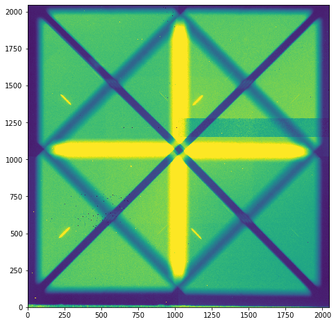
There are a few remaining artifacts in the image, but overall, not bad!
Now we can loop through all the files and calibrate them!
[9]:
######Set the calibration output directory. Set this up for your own group!!!#####
calib_dir = tutorial_dir+'/sample_data/'

unpol_calibrated_list = np.array([]) #This is a list of the calibrated files.

#Read in the file names
unpol_fnames  = asci.read(unpol_filelist , format = 'fast_no_header')['col1']
#source_fnames = asci.read(source_filelist, format = 'fast_no_header')['col1']

for i, fn in enumerate(unpol_fnames):
    #open the file
    raw_data = wo.wirc_data(raw_filename=unpol_fnames[i], flat_fn = flat_fn, dark_fn = dark_fn, bp_fn = bp_fn)
    #run the calibration
    raw_data.calibrate()
    #file name of the calibrated file
    outname = fn.split('.')[0]+'_calib.fits'
    #add to the list and save it
    unpol_calibrated_list = np.append(unpol_calibrated_list, calib_dir+outname)
    raw_data.save_wirc_object(calib_dir+outname)

###You may want to save the list, for late use, here's an example how:
# np.save(calib_dir+'unpol_calibrated_list.npy', unpol_calibrated_list)
Creating a new wirc_data object from file wirc0140.fits
Found a J-band filter in the header of file wirc0140.fits
Saving a wirc_object to /Users/maxwellmb/Dropbox (Personal)/Library/Python/wirc_drp/Tutorial/sample_data/wirc0140_calib.fits
Creating a new wirc_data object from file wirc0141.fits
Found a J-band filter in the header of file wirc0141.fits
Saving a wirc_object to /Users/maxwellmb/Dropbox (Personal)/Library/Python/wirc_drp/Tutorial/sample_data/wirc0141_calib.fits
Creating a new wirc_data object from file wirc0142.fits
Found a J-band filter in the header of file wirc0142.fits
Saving a wirc_object to /Users/maxwellmb/Dropbox (Personal)/Library/Python/wirc_drp/Tutorial/sample_data/wirc0142_calib.fits
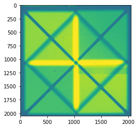
Now it’s your turn to set up a loop to calibrate the brown dwarf data!
[10]:
################ Brown Dwarf calibraton goes here ################

BD_calib_dir = tutorial_dir+'/sample_data/'

BD_calibrated_list = np.array([]) #This is a list of the calibrated files.

#First we'll set up all the directories and filenames:
BD_filelist = 'SIMP0136_sci.list' #for the source, the brown dwarf here

#Read in the file names
BD_fnames  = asci.read(BD_filelist , format = 'fast_no_header')['col1']
#source_fnames = asci.read(source_filelist, format = 'fast_no_header')['col1']

for i, fn in enumerate(BD_fnames):
    #open the file
    raw_data = wo.wirc_data(raw_filename=BD_fnames[i], flat_fn = flat_fn, dark_fn = dark_name60s_1, bp_fn = bp_fn)
    #run the calibration
    raw_data.calibrate(mask_bad_pixels=False)
    #file name of the calibrated file
    outname = fn.split('.')[0]+'_calib.fits'
    #add to the list and save it
    BD_calibrated_list = np.append(BD_calibrated_list, BD_calib_dir+outname)
    raw_data.save_wirc_object(BD_calib_dir+outname)

    plt.figure()
    plt.imshow(raw_data.full_image,vmax=10000)

###You may want to save the list, for late use, here's an example how:
# np.save(BD_calib_dir+'BD_calibrated_list.npy', BD_calibrated_list)
Creating a new wirc_data object from file wirc0158.fits
Found a J-band filter in the header of file wirc0158.fits
Saving a wirc_object to /Users/maxwellmb/Dropbox (Personal)/Library/Python/wirc_drp/Tutorial/sample_data/wirc0158_calib.fits
Creating a new wirc_data object from file wirc0159.fits
Found a J-band filter in the header of file wirc0159.fits
Saving a wirc_object to /Users/maxwellmb/Dropbox (Personal)/Library/Python/wirc_drp/Tutorial/sample_data/wirc0159_calib.fits
Creating a new wirc_data object from file wirc0160.fits
Found a J-band filter in the header of file wirc0160.fits
Saving a wirc_object to /Users/maxwellmb/Dropbox (Personal)/Library/Python/wirc_drp/Tutorial/sample_data/wirc0160_calib.fits
Step 2: Source identification
In this step we will create s wircpol_source object and attach it to each wirc_pol data object. Each source object will contain cutout thumbnails of each spectral trace, and eventually spectra and polarized spectra. We will then append the wircpol_source object to the wirc object’s “source_list”.
Again, we will show this step for one file first, then we will show steps 3-4 for this file. In the end we will loop through and do this for every file.
[11]:
#First we'll create a new data object, mostly just to demonstrate how to read in an existing wirc_data object.
calibrated_data = wo.wirc_data(wirc_object_filename=BD_calibrated_list[1])
Loading a wirc_data object from file /Users/maxwellmb/Dropbox (Personal)/Library/Python/wirc_drp/Tutorial/sample_data/wirc0159_calib.fits
Generate a background image by scaling the “calibrated” image from the _Single_File tutorial
[12]:
calibrated_data.generate_bkg(method="scaled_bkg",bkg_fns=[tutorial_dir+"/calibrated.fits"],same_HWP=False)
Put in the coordinates of the source here, then add source to the wirc_data object
[13]:
source_coords = [700, 955] #X, Y position of the zeroth order of the source (undispersed star in the center)

# This function add the source to our wirc_data object created in the last cell.
# update_w_chi2_shift flag centers the source
calibrated_data.add_source( source_coords[0], source_coords[1],
                slit_pos = "slitless", update_w_chi2_shift = True, verbose = True)

# We can access the source from the source list attribute
wp_source = calibrated_data.source_list[0]
Loading Template from /Users/maxwellmb/Dropbox (Personal)/Library/Python/wirc_drp/wirc_drp/masks/single_trace_template2.fits
Shfits are x,y =  [3.314453125, 1.751953125, 0.052734375, 0.052734375]
Applying shifts
/Users/maxwellmb/Dropbox (Personal)/Library/Python/image_registration/build/lib.macosx-10.7-x86_64-3.7/image_registration/fft_tools/zoom.py:101: FutureWarning: Using a non-tuple sequence for multidimensional indexing is deprecated; use `arr[tuple(seq)]` instead of `arr[seq]`. In the future this will be interpreted as an array index, `arr[np.array(seq)]`, which will result either in an error or a different result.
  outarr[ii] = outarr_d[dims]
We’ll now get the trace cutouts for this source
[14]:
wp_source.get_cutouts(calibrated_data.full_image, calibrated_data.DQ_image, calibrated_data.filter_name,
                      calibrated_data.bkg_image, replace_bad_pixels = True, sub_bar = True, cutout_size = 75)
Source 1's traces will hit the vertical bar of doom, compensating by subtracting the median of the edges of each row
Source 1's traces will hit the vertical bar of doom, compensating by subtracting the median of the edges of each row
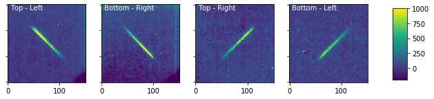
Plot the cutouts
[15]:
wp_source.plot_cutouts(figsize=(10,6),vmin=-200,vmax=1000)
Plot the background-subtracted cutouts
[16]:
wp_source.plot_cutouts(figsize=(10,6),plot_bkg_sub=True,vmin=-500,vmax=500)
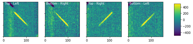
This background subtraction has clearly introduced some features into the image that aren’t ideal, but in a real observation set you will have taken more appropriate background images. There are also several different background subgraction options that you can experiment with within the wircpol_data.generate_bkg() functions that may improve your results.
Step 3-4: Background subtraction and spectral extraction
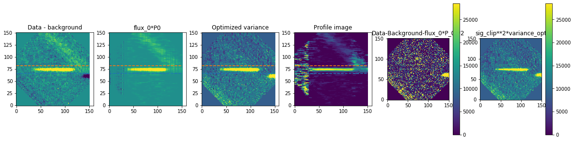
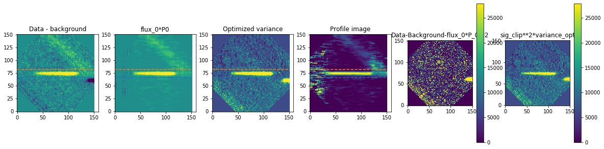
In this step we will subtract background and extract the specta from one of the source objects we found in Step 2. Options for the spectral extraction function are pretty extensive, but here are all you need to care about:
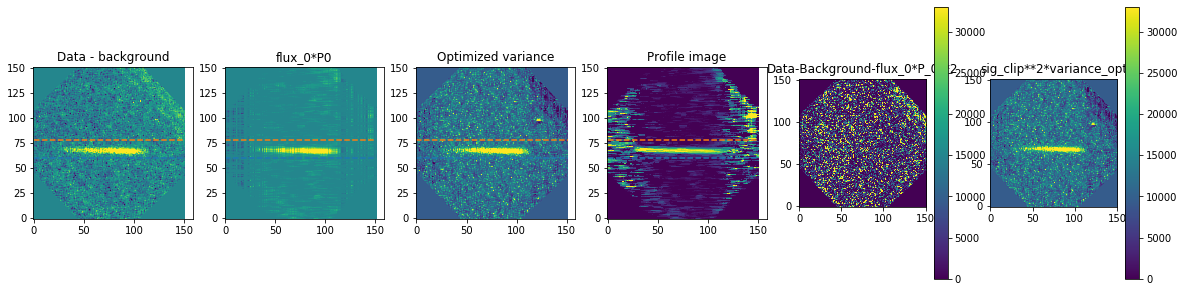
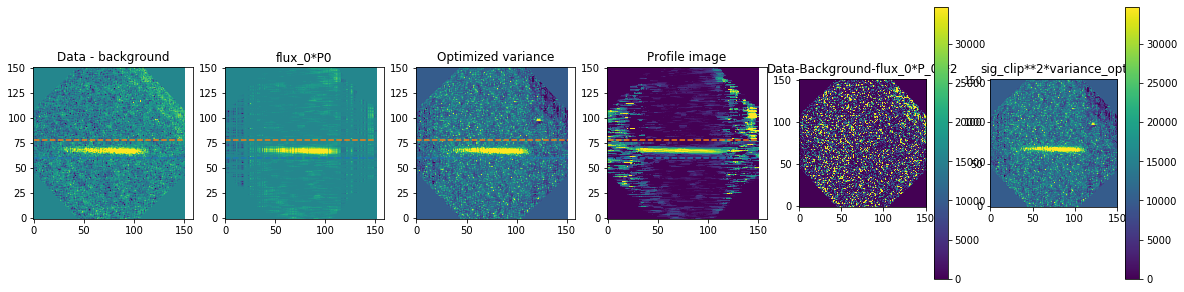
method is how we exactly extract the spectra. We are using optimal extraction here and you can read about it in Horne 1986. spatial_sigma is how far in the wings of the spectral trace we want to extract.
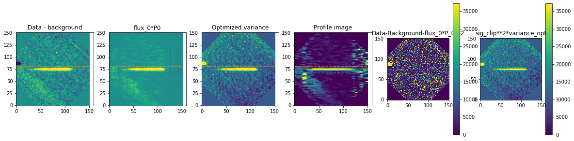
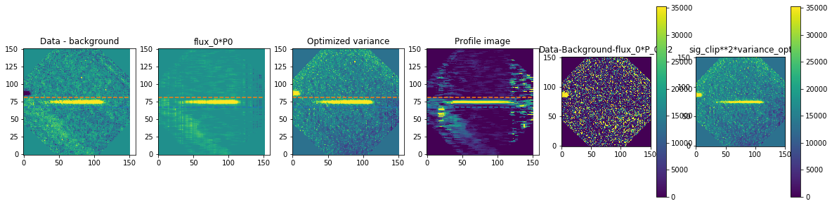
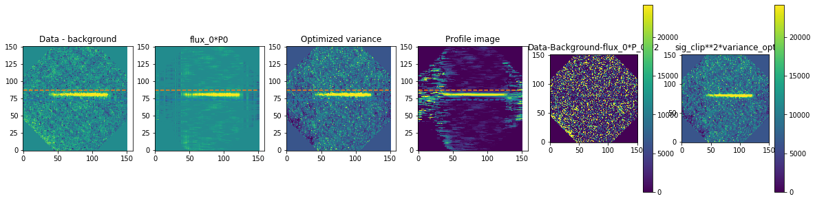
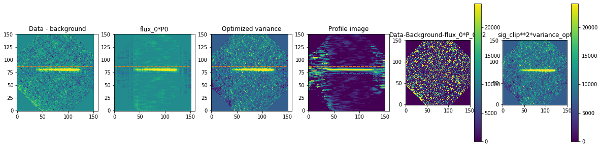
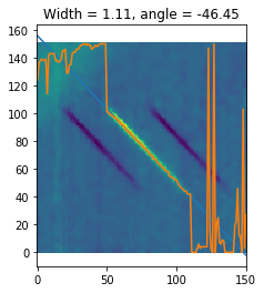
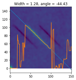
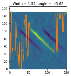
Here we’ll plot some of the internal workings for each trace. Each trace goes through 2 iterations of the optimal extraction algorithm. The orange and blue lines show the regions defined by the spatial_sigma parameter.
[17]:
calibrated_data.source_list[0].extract_spectra(method="optimal_extraction",
spatial_sigma=4,
bad_pix_masking = 1,
plot_optimal_extraction = True,
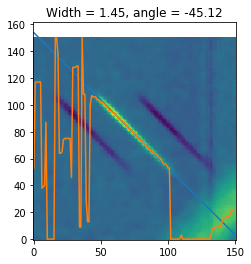
plot_findTrace = False,
verbose=False)
Now let’s plot the spectra:
[18]:
calibrated_data.source_list[0].plot_trace_spectra()
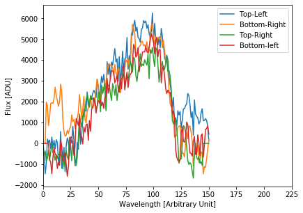
It is clear that these spectra are messed up, and it’s related to the background levels. This is a work in progress (and one of the reasons we suggest that you don’t use your data for science without talking to the instrument team).
Now with Steps 2-4 demonstrated for one file, let’s run it all on all files: First with the unpolarized standard star
[19]:
source_list = []
all_spec_cube = []
counter = 0
for i,fn in enumerate(unpol_calibrated_list):
    try:
        print("Extracting from file {} of {}".format(counter+1, len(unpol_calibrated_list)))
        data = wo.wirc_data(wirc_object_filename=fn, verbose=False)
        im = np.array(data.full_image).copy()

        data.generate_bkg()

        #Clear the source list
        data.source_list = []
        data.n_sources = 0
        data.add_source( source_coords[0], source_coords[1], slit_pos = "slitless",
                        update_w_chi2_shift = True, verbose = False)

        #Let's save ourselves from million plots
        do_plot = False
        #Get cutouts of the 4 spectra and plot them for every 10 frames
        data.source_list[0].get_cutouts(data.full_image, data.DQ_image, data.filter_name, data.bkg_image,
                                        replace_bad_pixels = True,
                                        sub_bar = True, cutout_size = 75)
#         if do_plot == True:
#             data.source_list[0].plot_cutouts(origin ='lower')
        #Now extract the spectra
        data.source_list[0].extract_spectra(method="optimal_extraction",
                                   bad_pix_masking =1,
                                   plot_optimal_extraction = False,
                                    plot_findTrace = do_plot,
                                   verbose=False, spatial_sigma=10)
        #Save the spectra in this array
        all_spec_cube.append(data.source_list[0].trace_spectra)
        #Save the file
        data.save_wirc_object(fn)
        source_list += [data.source_list[0]]
    except Exception as e:
        print("Some sort of Error, skipping file {}".format(fn))
        print("Error {}".format(e))
    counter += 1
# trace_info = iu.locate_traces(im,sky, plot=False, verbose=True)

source_list = copy.deepcopy(source_list)
up_all_spec_cube = np.array(all_spec_cube)
Extracting from file 1 of 3
Subtracting background using shift and subtract method.
Applying shifts
Source 1's traces will hit the vertical bar of doom, compensating by subtracting the median of the edges of each row
Source 1's traces will hit the vertical bar of doom, compensating by subtracting the median of the edges of each row
Saving a wirc_object to /Users/maxwellmb/Dropbox (Personal)/Library/Python/wirc_drp/Tutorial/sample_data/wirc0140_calib.fits
WARNING: VerifyWarning: Card is too long, comment will be truncated. [astropy.io.fits.card]
Extracting from file 2 of 3
Subtracting background using shift and subtract method.
Applying shifts
Source 1's traces will hit the vertical bar of doom, compensating by subtracting the median of the edges of each row
Source 1's traces will hit the vertical bar of doom, compensating by subtracting the median of the edges of each row
Saving a wirc_object to /Users/maxwellmb/Dropbox (Personal)/Library/Python/wirc_drp/Tutorial/sample_data/wirc0141_calib.fits
Extracting from file 3 of 3
Subtracting background using shift and subtract method.
Applying shifts
Source 1's traces will hit the vertical bar of doom, compensating by subtracting the median of the edges of each row
Source 1's traces will hit the vertical bar of doom, compensating by subtracting the median of the edges of each row
Saving a wirc_object to /Users/maxwellmb/Dropbox (Personal)/Library/Python/wirc_drp/Tutorial/sample_data/wirc0142_calib.fits
Then the brown dwarf
[20]:
source_list = []
BD_all_spec_cube = []
counter = 0
for i,fn in enumerate(BD_calibrated_list):
    try:
        print("Extracting from file {} of {}".format(counter+1, len(BD_calibrated_list)))
        data = wo.wirc_data(wirc_object_filename=fn, verbose=False)
        data.generate_bkg()
        im = np.array(data.full_image).copy()
        #Clear the source list
        data.source_list = []
        data.n_sources = 0
        data.add_source( source_coords[0], source_coords[1], slit_pos = "slitless",
                        update_w_chi2_shift = True, verbose = False)
        #Let's save ourselves from million plots
        if i%10 == 0:
            do_plot = True
        else:
            do_plot = False

        #Get cutouts of the 4 spectra and plot them for every 10 frames
        data.source_list[0].get_cutouts(data.full_image, data.DQ_image, data.filter_name, data.bkg_image,
                                        replace_bad_pixels = True,
                                        sub_bar = True, cutout_size = 75)
#         if do_plot == True:
#             data.source_list[0].plot_cutouts(origin ='lower')
        #Now extract the spectra
        data.source_list[0].extract_spectra(method="optimal_extraction",
                                   bad_pix_masking =1,
                                   plot_optimal_extraction = False,
                                    plot_findTrace = do_plot,
                                   verbose=False, spatial_sigma=10)
        #Save the spectra in this array
        BD_all_spec_cube.append(data.source_list[0].trace_spectra)
        #Save the file
        data.save_wirc_object(fn)
        source_list += [data.source_list[0]]
    except Exception as e:
        print("Some sort of Error, skipping file {}".format(fn))
        print("Error {}".format(e))
    counter += 1
# trace_info = iu.locate_traces(im,sky, plot=False, verbose=True)

source_list = copy.deepcopy(source_list)
BD_up_all_spec_cube = np.array(BD_all_spec_cube)
Extracting from file 1 of 3
Subtracting background using shift and subtract method.
Applying shifts
Source 1's traces will hit the vertical bar of doom, compensating by subtracting the median of the edges of each row
Source 1's traces will hit the vertical bar of doom, compensating by subtracting the median of the edges of each row
Saving a wirc_object to /Users/maxwellmb/Dropbox (Personal)/Library/Python/wirc_drp/Tutorial/sample_data/wirc0158_calib.fits
Extracting from file 2 of 3
Subtracting background using shift and subtract method.
Applying shifts
Source 1's traces will hit the vertical bar of doom, compensating by subtracting the median of the edges of each row
Source 1's traces will hit the vertical bar of doom, compensating by subtracting the median of the edges of each row
Saving a wirc_object to /Users/maxwellmb/Dropbox (Personal)/Library/Python/wirc_drp/Tutorial/sample_data/wirc0159_calib.fits
Extracting from file 3 of 3
Subtracting background using shift and subtract method.
Applying shifts
Source 1's traces will hit the vertical bar of doom, compensating by subtracting the median of the edges of each row
Source 1's traces will hit the vertical bar of doom, compensating by subtracting the median of the edges of each row
Saving a wirc_object to /Users/maxwellmb/Dropbox (Personal)/Library/Python/wirc_drp/Tutorial/sample_data/wirc0160_calib.fits
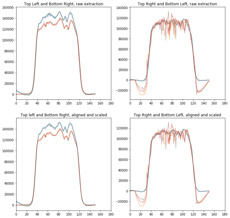
Step 5 - Stack the spectra
Here we simply align spectra from all the exposures, scale and median combine them.
[21]:
#Align the spectra.
up_aligned_cube = su.align_spectral_cube(up_all_spec_cube)

#Scale the spectra to compensate for atmospheric variation - you may not want to do this all the time
up_scaled_cube = su.scale_and_combine_spectra(up_aligned_cube, return_scaled_cube = True)
[22]:
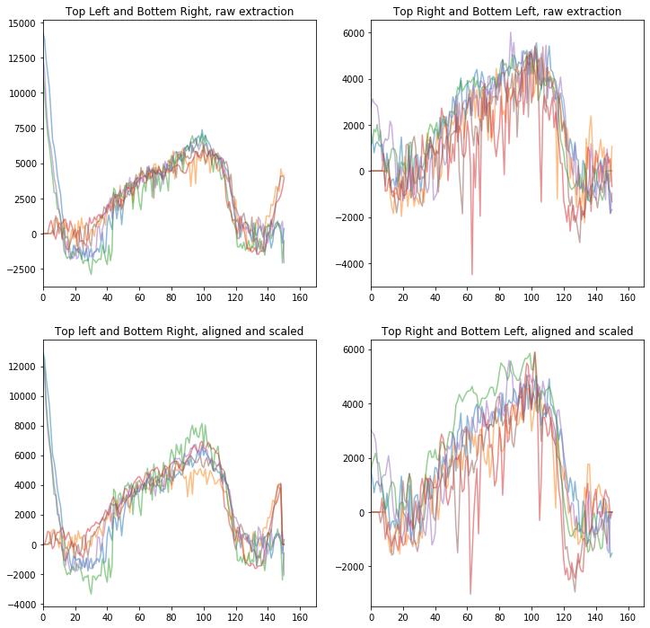
#Plot them. The top plots are raw extraction, bottom are aligned and scaled.
#The left plots are upper left, lower right (U pair), and right plots are Q pair.
### What do the spectra look like
fig, ax = plt.subplots(2,2,figsize=(12,12))
low_ind =  0
high_ind = 180

cm1 = plt.get_cmap('bwr')
cm2 = plt.get_cmap('copper')
alpha = 0.5

for i in range(up_all_spec_cube.shape[0]):
    ax[0,0].plot(up_all_spec_cube[i,0,1,:], alpha = alpha) #top left
    ax[0,0].plot(up_all_spec_cube[i,1,1,:], alpha = alpha) #bottom right
    ax[0,1].plot(up_all_spec_cube[i,2,1,:], alpha = alpha) #top right
    ax[0,1].plot(up_all_spec_cube[i,3,1,:], alpha = alpha) #bottom left

    #aligned and scaled cube
    ax[1,0].plot(up_scaled_cube[i,0,1,:], alpha = alpha) #top left
    ax[1,0].plot(up_scaled_cube[i,1,1,:], alpha = alpha) #bottom right
    ax[1,1].plot(up_scaled_cube[i,2,1,:], alpha = alpha) #top right
    ax[1,1].plot(up_scaled_cube[i,3,1,:], alpha = alpha) #bottom left

ax[0,0].set_xlim([low_ind, high_ind])
ax[0,1].set_xlim([low_ind, high_ind])
ax[1,0].set_xlim([low_ind, high_ind])
ax[1,1].set_xlim([low_ind, high_ind])
# ax[0,0].set_ylim([0, 180000])
# ax[0,1].set_ylim([0, 150000])
# ax[1,0].set_ylim([0, 180000])
# ax[1,1].set_ylim([0, 150000])


ax[0,0].set_title('Top Left and Bottom Right, raw extraction')
ax[0,1].set_title('Top Right and Bottom Left, raw extraction')
ax[1,0].set_title('Top left and Bottom Right, aligned and scaled')
ax[1,1].set_title('Top Right and Bottom Left, aligned and scaled')
[22]:
Text(0.5, 1.0, 'Top Right and Bottom Left, aligned and scaled')
We can now median combine and compute standard deviation of the measurement.
The most manual step here is to make sure the 4 spectra are aligned in wavelength, this is caused by the tilt of the J-band filter. The offsets given below are good, but let’s plot them to check.
[23]:
sshift_um = 0
sshift_up = -2.2
sshift_qm = +0.7
sshift_qp = -2.5

unpol_um_med = shift(np.nanmedian(up_scaled_cube[:,0,1,:], axis=0),sshift_um, order = 1)
unpol_up_med = shift(np.nanmedian(up_scaled_cube[:,1,1,:], axis=0),sshift_up, order = 1)
unpol_qm_med = shift(np.nanmedian(up_scaled_cube[:,2,1,:], axis=0),sshift_qm, order = 1)
unpol_qp_med = shift(np.nanmedian(up_scaled_cube[:,3,1,:], axis=0),sshift_qp, order = 1)

unpol_um_std = shift(np.nanstd(up_scaled_cube[:,0,1,:], axis=0)/np.sqrt(up_scaled_cube.shape[0]),sshift_um, order = 1)
unpol_up_std = shift(np.nanstd(up_scaled_cube[:,1,1,:], axis=0)/np.sqrt(up_scaled_cube.shape[0]),sshift_up, order = 1)
unpol_qm_std = shift(np.nanstd(up_scaled_cube[:,2,1,:], axis=0)/np.sqrt(up_scaled_cube.shape[0]),sshift_qm, order = 1)
unpol_qp_std = shift(np.nanstd(up_scaled_cube[:,3,1,:], axis=0)/np.sqrt(up_scaled_cube.shape[0]),sshift_qp, order = 1)
[24]:
plt.figure(figsize = (7.5,7.5))
vector = [unpol_qp_med,unpol_qm_med,unpol_up_med,unpol_um_med]
labels = ['Qp','Qm','Up','Um']
factors = np.sum(unpol_qp_med[50:110])/np.array([np.sum(x[50:110]) for x in vector])
factors[1] = factors[1]*1.015
factors[2] = factors[2]*0.995
factors[3] = factors[3]*1.005
fmts =   ['-b','-r','--b','--r']
for i in range(len(vector)):
    plt.plot(vector[i]*factors[i],fmts[i], label = labels[i])
# plt.xlim([low_ind, high_ind])
plt.xlim([low_ind, high_ind])
plt.xlim([0,180])
#plt.ylim([100000,140000])
plt.xlabel('Spectral pixel')
plt.ylabel('Counts')
plt.legend()
plt.title('Four traces of unpolarized standard')
[24]:
Text(0.5, 1.0, 'Four traces of unpolarized standard')
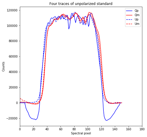
Each trace corresponds to Stokes parameters as following: Qp – Bottom left; Qm – Top right; Up – Bottom right; Um – Top left.
These are such that normalized Stokes parameters are q = (Qp - Qm)/(Qp + Qm) and u = (Up - Um)/(Up + Um)
Now do the same for the brown dwarf
[25]:
BD_up_aligned_cube = su.align_spectral_cube(BD_up_all_spec_cube)
BD_up_scaled_cube = su.scale_and_combine_spectra(BD_up_aligned_cube, return_scaled_cube = True)

fig1, ax1 = plt.subplots(2,2,figsize=(12,12))
low_ind =  0
high_ind = 170

cm1 = plt.get_cmap('bwr')
cm2 = plt.get_cmap('copper')
alpha = 0.5

for i in range(BD_up_all_spec_cube.shape[0]):
    ax1[0,0].plot(BD_up_all_spec_cube[i,0,1,:], alpha = alpha) #top left
    ax1[0,0].plot(BD_up_all_spec_cube[i,1,1,:], alpha = alpha) #bottom right
    ax1[0,1].plot(BD_up_all_spec_cube[i,2,1,:], alpha = alpha) #top right
    ax1[0,1].plot(BD_up_all_spec_cube[i,3,1,:], alpha = alpha) #bottom left

    #aligned and scaled cube
    ax1[1,0].plot(BD_up_scaled_cube[i,0,1,:], alpha = alpha) #top left
    ax1[1,0].plot(BD_up_scaled_cube[i,1,1,:], alpha = alpha) #bottom right
    ax1[1,1].plot(BD_up_scaled_cube[i,2,1,:], alpha = alpha) #top right
    ax1[1,1].plot(BD_up_scaled_cube[i,3,1,:], alpha = alpha) #bottom left

ax1[0,0].set_xlim([low_ind, high_ind])
ax1[0,1].set_xlim([low_ind, high_ind])
ax1[1,0].set_xlim([low_ind, high_ind])
ax1[1,1].set_xlim([low_ind, high_ind])
#ax1[0,0].set_ylim([0, 180000])
#ax1[0,1].set_ylim([0, 150000])
#ax1[1,0].set_ylim([0, 180000])
#ax1[1,1].set_ylim([0, 150000])


ax1[0,0].set_title('Top Left and Bottem Right, raw extraction')
ax1[0,1].set_title('Top Right and Bottem Left, raw extraction')
ax1[1,0].set_title('Top left and Bottem Right, aligned and scaled')
ax1[1,1].set_title('Top Right and Bottem Left, aligned and scaled')
[25]:
Text(0.5, 1.0, 'Top Right and Bottem Left, aligned and scaled')
[26]:
#now shifts for the BD spectra
sshift_um = 0
sshift_up = -2.2
sshift_qm = +0.7
sshift_qp = +1
BD_um_med = shift(np.nanmedian(BD_up_scaled_cube[:,0,1,:], axis=0),sshift_um, order = 1)
BD_up_med = shift(np.nanmedian(BD_up_scaled_cube[:,1,1,:], axis=0),sshift_up, order = 1)
BD_qm_med = shift(np.nanmedian(BD_up_scaled_cube[:,2,1,:], axis=0),sshift_qm, order = 1)
BD_qp_med = shift(np.nanmedian(BD_up_scaled_cube[:,3,1,:], axis=0),sshift_qp, order = 1)
BD_um_std = shift(np.nanstd(BD_up_scaled_cube[:,0,1,:], axis=0)/np.sqrt(BD_up_scaled_cube.shape[0]),sshift_um, order = 1)
BD_up_std = shift(np.nanstd(BD_up_scaled_cube[:,1,1,:], axis=0)/np.sqrt(BD_up_scaled_cube.shape[0]),sshift_up, order = 1)
BD_qm_std = shift(np.nanstd(BD_up_scaled_cube[:,2,1,:], axis=0)/np.sqrt(BD_up_scaled_cube.shape[0]),sshift_qm, order = 1)
BD_qp_std = shift(np.nanstd(BD_up_scaled_cube[:,3,1,:], axis=0)/np.sqrt(BD_up_scaled_cube.shape[0]),sshift_qp, order = 1)
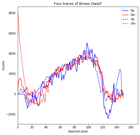
plt.figure(figsize = (7.5,7.5))
vector = [BD_qp_med,BD_qm_med,BD_up_med,BD_um_med]
labels = ['Qp','Qm','Up','Um']
factors = np.sum(BD_qp_med[40:120])/np.array([np.sum(x[40:120]) for x in vector])
factors[1] = factors[1]*1.015
factors[2] = factors[2]*0.995
factors[3] = factors[3]*1.005
fmts = ['-b','-r','--b','--r']
for i in range(len(vector)):
plt.plot(vector[i]*factors[i],fmts[i], label = labels[i])
# plt.xlim([low_ind, high_ind])
plt.xlim([low_ind, high_ind])
#plt.xlim([160,180])
#plt.ylim([100000,140000])
plt.xlabel('Spectral pixel')
plt.ylabel('Counts')
plt.legend()
plt.title('Four traces of Brown Dwarf')
[26]:
Text(0.5, 1.0, 'Four traces of Brown Dwarf')
Let’s now save out spectra to a numpy file.
[27]:
np.save("BD_Spectra",BD_up_scaled_cube)
Step 6: Polarization calibration and calculation
Note, that if you’re using data from after March 2019 that uses the new awesome half-wave plate, then instead of reading this section, you should move on to the other tutorial: WIRC+Pol_Tutorial_3-Reducing_a_Modulation_Sequence
Suggestions: The most crucial part here is to get wavelength to line up. This is a bit tricky since WIRC+Pol is slitless and there’s no easy way to get wavelength solution directly from the data.
We suggest that you align the brown dwarf spectra to those of the standard star trace by trace relying on the filter cutoffs. Note that different traces have difference filter cutoff.
From the last part, you would have the median spectra: unpol_qp_med, unpol_qm_med and pol_qp_med, pol_qm_med from the standard and the brown dwarf respectively.
[28]:
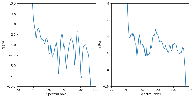
#First compute q, u from the unpolarized star. This is the instrumental polarization
import math
import numpy as np

q_inst = (unpol_qp_med - unpol_qm_med)/(unpol_qp_med + unpol_qm_med)
u_inst = (unpol_up_med - unpol_um_med)/(unpol_up_med + unpol_um_med)

# Uncertainties, fill this in!

q_inst_err = 2/(unpol_qp_med+unpol_qm_med)**2*np.sqrt((unpol_qp_med*unpol_qm_std)**2 + (unpol_qm_med*unpol_qp_std)**2 )
u_inst_err = 2/(unpol_up_med+unpol_um_med)**2*np.sqrt((unpol_up_med*unpol_um_std)**2 + (unpol_um_med*unpol_up_std)**2 )
/Users/maxwellmb/Anaconda3/anaconda3/lib/python3.7/site-packages/ipykernel_launcher.py:5: RuntimeWarning: invalid value encountered in true_divide
  """
/Users/maxwellmb/Anaconda3/anaconda3/lib/python3.7/site-packages/ipykernel_launcher.py:6: RuntimeWarning: invalid value encountered in true_divide

/Users/maxwellmb/Anaconda3/anaconda3/lib/python3.7/site-packages/ipykernel_launcher.py:10: RuntimeWarning: divide by zero encountered in true_divide
  # Remove the CWD from sys.path while we load stuff.
/Users/maxwellmb/Anaconda3/anaconda3/lib/python3.7/site-packages/ipykernel_launcher.py:10: RuntimeWarning: invalid value encountered in multiply
  # Remove the CWD from sys.path while we load stuff.
/Users/maxwellmb/Anaconda3/anaconda3/lib/python3.7/site-packages/ipykernel_launcher.py:11: RuntimeWarning: divide by zero encountered in true_divide
  # This is added back by InteractiveShellApp.init_path()
/Users/maxwellmb/Anaconda3/anaconda3/lib/python3.7/site-packages/ipykernel_launcher.py:11: RuntimeWarning: invalid value encountered in multiply
  # This is added back by InteractiveShellApp.init_path()
[29]:
#show this

fig, ax = plt.subplots(1,2, figsize = (10,5))
ax[0].plot(q_inst*100)
ax[1].plot(u_inst*100)

ax[0].set_xlim([20,120])
ax[1].set_xlim([20,120])
ax[0].set_ylim([-10,10])
ax[1].set_ylim([-10,0])

ax[0].set_xlabel('Spectral pixel')
ax[1].set_xlabel('Spectral pixel')

ax[0].set_ylabel('q (%)')
ax[1].set_ylabel('u (%)')
[29]:
Text(0, 0.5, 'u (%)')
[30]:
#### Do the same for the Brown Dwarf ####
[31]:
q_BD_raw = (BD_qp_med - BD_qm_med)/(BD_qp_med + BD_qm_med)
u_BD_raw = (BD_up_med - BD_um_med)/(BD_up_med + BD_um_med)

# Uncertainties, fill this in!

q_BD_raw_err = 2/(BD_qp_med+BD_qm_med)**2*np.sqrt((BD_qp_med*BD_qm_std)**2 + (BD_qm_med*BD_qp_std)**2 )
u_BD_raw_err = 2/(BD_up_med+BD_um_med)**2*np.sqrt((BD_up_med*BD_um_std)**2 + (BD_um_med*BD_up_std)**2 )

#Now subtract the instrumental polarization
q_BD_corrected =  q_BD_raw - q_inst
u_BD_corrected =  u_BD_raw - u_inst

q_BD_corrected_err = np.sqrt(q_BD_raw_err**2 + q_inst_err**2)
u_BD_corrected_err = np.sqrt(u_BD_raw_err**2 + u_inst_err**2)
/Users/maxwellmb/Anaconda3/anaconda3/lib/python3.7/site-packages/ipykernel_launcher.py:1: RuntimeWarning: invalid value encountered in true_divide
  """Entry point for launching an IPython kernel.
/Users/maxwellmb/Anaconda3/anaconda3/lib/python3.7/site-packages/ipykernel_launcher.py:6: RuntimeWarning: divide by zero encountered in true_divide

/Users/maxwellmb/Anaconda3/anaconda3/lib/python3.7/site-packages/ipykernel_launcher.py:6: RuntimeWarning: invalid value encountered in multiply
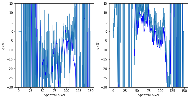
[32]:
### Plot q_BD_raw, q_BD_corrected here

fig, ax = plt.subplots(1,2, figsize = (10,5))

x = range(len(q_BD_raw))
ax[0].plot(x,q_BD_raw*100,'-b')
#ax[0].plot(q_BD_corrected*100,'-r')

ax[1].plot(x,u_BD_raw*100,'b-')
#ax[1].plot(u_BD_corrected*100,'-r')

#ax[0].set_xlim([100,200])
#ax[1].set_xlim([100,200])
ax[0].set_ylim([-30,15])
ax[1].set_ylim([-30,15])

ax[0].set_xlabel('Spectral pixel')
ax[1].set_xlabel('Spectral pixel')

ax[0].set_ylabel('q (%)')
ax[1].set_ylabel('u (%)')

#q here
ax[0].errorbar(x,q_BD_corrected*100,yerr=q_BD_corrected_err*100)
#u here
ax[1].errorbar(x,u_BD_corrected*100,yerr=u_BD_corrected_err*100)
[32]:
<ErrorbarContainer object of 3 artists>
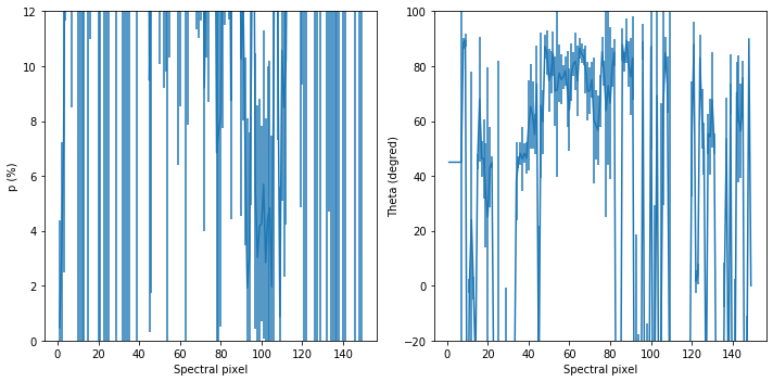
[33]:
#### Finally, compute degree and angle of polarization

p = np.sqrt(q_BD_corrected**2 + u_BD_corrected**2)
theta = 0.5*np.arctan2(u_BD_corrected, q_BD_corrected)

#uncertainties

p_err = (1/p)*np.sqrt((q_BD_corrected*q_BD_corrected_err)**2 + (u_BD_corrected*u_BD_corrected_err)**2)
# theta_err = (0.5/(1+(u_BD_corrected/q_BD_corrected)**2))*np.sqrt((u_BD_corrected_err/q_BD_corrected)**2 + (u_BD_corrected*q_BD_corrected_err/(q_BD_corrected**2))**2)
theta_err = (0.5/p**2)*np.sqrt((q_BD_corrected*u_BD_corrected_err)**2 + (u_BD_corrected*q_BD_corrected_err)**2)

#plot these!

fig, ax = plt.subplots(1,2, figsize = (10,5))

x = range(len(q_BD_raw))
# ax[0].plot(x,p*100,'-b')
# ax[1].plot(x,theta,'b-')
#ax[1].plot(u_BD_corrected*100,'-r')

#ax[0].set_xlim([100,200])
#ax[1].set_xlim([100,200])
ax[0].set_ylim([-0,12])
ax[1].set_ylim([-20,100])

ax[0].set_xlabel('Spectral pixel')
ax[1].set_xlabel('Spectral pixel')

ax[0].set_ylabel('p (%)')
ax[1].set_ylabel('Theta (degred)')

#q here
ax[0].errorbar(x,p*100,yerr=p_err*100)
#u here
ax[1].errorbar(x,np.degrees(theta),yerr=np.degrees(theta_err))
plt.tight_layout()
/Users/maxwellmb/Anaconda3/anaconda3/lib/python3.7/site-packages/ipykernel_launcher.py:8: RuntimeWarning: divide by zero encountered in true_divide

/Users/maxwellmb/Anaconda3/anaconda3/lib/python3.7/site-packages/ipykernel_launcher.py:8: RuntimeWarning: invalid value encountered in multiply

/Users/maxwellmb/Anaconda3/anaconda3/lib/python3.7/site-packages/ipykernel_launcher.py:10: RuntimeWarning: divide by zero encountered in true_divide
  # Remove the CWD from sys.path while we load stuff.
/Users/maxwellmb/Anaconda3/anaconda3/lib/python3.7/site-packages/ipykernel_launcher.py:10: RuntimeWarning: invalid value encountered in multiply
  # Remove the CWD from sys.path while we load stuff.
Acknowledgement
The data used in this Tutorial are taken by the Ay122a class in Fall 2018 with Prof. Dimitri Mawet. Class members are Aida, Anise, Anusha, Luiza, Nitika, Ryan, Yuhan, Yuping, Zhihui, and TA Jackie Pezzato. They contributed to making this Tutorial as well.
[ ]:
[ ]: